Building An Inductive Representation of SSA

Published: 2024-07-21

Static Single Assignment form, or SSA, is the intermediate representation of choice for designing compilers for a vast variety of languages and platforms. SSA, however, is usually cast in a very “imperative” style, making it difficult to take advantage of functional programming when writing optimizations and analyses, and extremely cumbersome to reason about effectively in a theorem prover. In this article, we discuss how we might work towards a more “functional,” and in particular inductive, representation of SSA. In particular, we will discuss representations of SSA inside the Lean theorem prover which I have developed over the course of my research, from a formalization of “vanilla” 3-address code and SSA in freyd-ssa to my work on inductive representations of SSA in debruijn-ssa.

Classical SSA

We begin by telling the story of freyd-ssa, our attempt to formalize classical SSA mostly as is and prove some theorems. This is still very work-in-progress and mostly abandoned, but it is sorry-free, and while it does not by any means follow best practices, designing it was very educational!

A Type System for 3-address code

In 3 address code, a program is decomposed into a control-flow graph made up of basic blocks. For example, this C program:

int f(int a, int b, int c) {
    int p = a + 5;
    int q = b + p;
    for (int i = 0; i < q; i++) {
        p += i + c;
        if (p % 3 == 0) {
            p += 2;
        }
    }
    return p;
}

might become

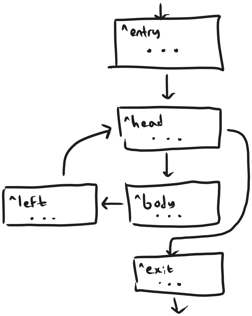
^entry:
    p = a + 5;
    q = b + p;
    i = 0;
    br ^head
^head:
    ite (i < q) ^exit ^body
^body:
    i = i + 1;
    t = i + c;
    p = p + t;
    ite (p % 3) ^tt ^head
^tt:
    p = p + 2;
    br ^head
^exit:
    ret p

or, drawn as a graph,

In general, a program in three-adress code is composed of:

• A control-flow graph, composed from a set of entries, exists, and
• Basic blocks, which are defined as a linear sequence of instructions (the body) followed by a terminator.

More formally, let’s consider instructions $f: A_1 \times ... \times A_n \to B_1 \times ... \times B_m$ taking in $n$ parameters $a_1,...,a_n$ and returning $m$ outputs of type $B_1,..., B_m$. For convenience, we will simply write such bundles of parameters as $f : (A_i)_i \to (B_j)_j$.

We might begin by giving a typing judgement for bodies:

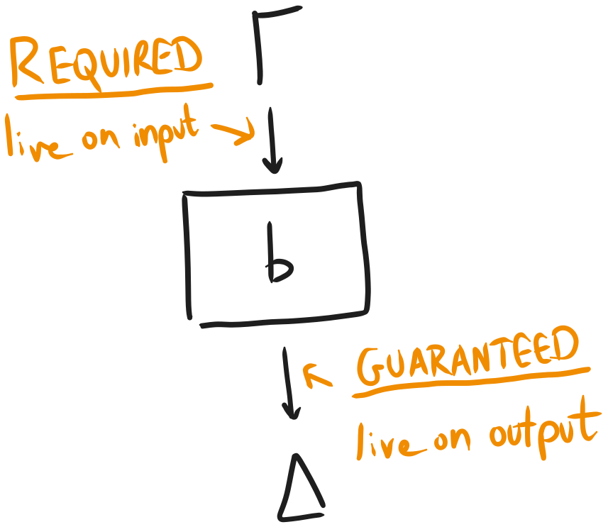
$\Gamma \vdash b : \Delta$ means that if the variables in the context $\Gamma$ are live on input to $b$, then the variables in the context $\Delta$ will be live once the instructions in $b$ are finished executing.

Here, a context is just a (finitely-supported) partial function from variables to types; the domain of this function is our live variable set.

We can give typing rules

Let’s break this down:

• $\Gamma \leq \Delta$ denotes that $\Gamma$ weakens $\Delta$, i.e., that if $\Gamma(x) = A$, then $\Delta(x) = A$. So the first rule says that the empty body, $\cdot$, which just does nothing, is allowed to throw away unused live variables in the input, but that’s it.
• $\Gamma, x: A$ denotes updating $\Gamma(x)$ to $A$ (whether or not it was previously defined). So the second rule says that if $b$ takes inputs $\Gamma, (y_j : B_j)_j$ to $\Delta$, then first updating $(y_j)_j$ to be the outputs of $f (x_i)_i$ and then executing $b$ takes $\Gamma$ to $\Delta$, assuming that $\Gamma$ types each $x_i$ correctly to be an input of $f$.

For a quick sanity check, we can verify that this definition satisfies weakening on both the left and right:

We can also prove a variant of the frame rule (assuming all variables in $\Xi$ are fresh!):

A basic block, given a set of live variables on input, executes its body and then jumps to another basic block via its terminator (for simplicity, we can model returns as jumping to a special “return” label). We might represent this using the judgement

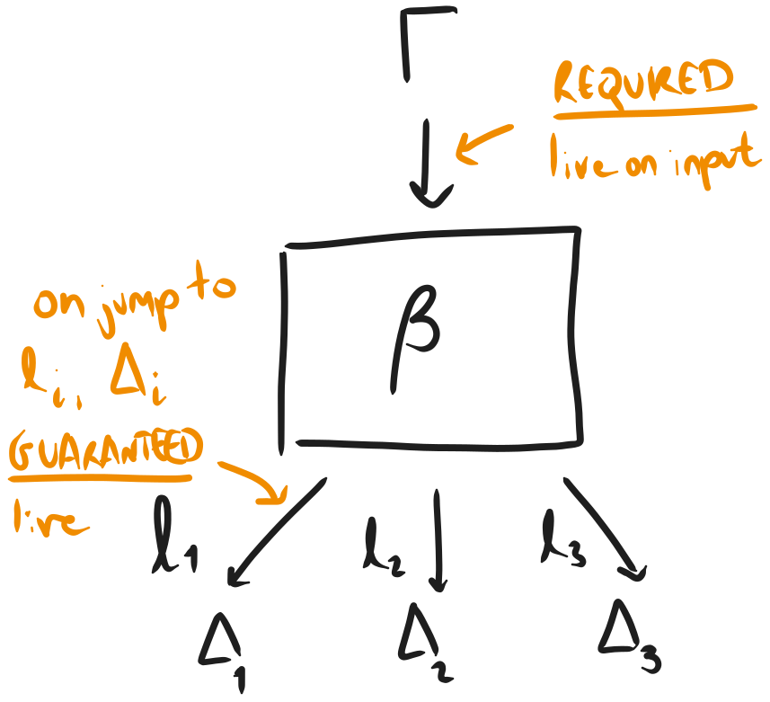
Just like before, $\Gamma$ is the set of live variables on entry to the basic block $\beta$. On the other hand, $\mathcal{L}$ is a label context: a finitely supported map from labels $\ell$ to contexts $\Gamma$, which represent the variables which must be live on entry to $\ell$, as below:

We might give the following simple typing rules for basic blocks

In other words, as one would expect, a basic block consists of a body followed by a terminator; with the latter being either an unconditional branch ($\mathsf{br}$) or a conditional branch ($\mathsf{ite}$). The body transforms the variables required live on input, $\Gamma$, into the variables guaranteed live on output, $\Delta$; the conditions for terminators state that, for all possible output labels $\ell$, $\Delta$ is a weakening of the variables required for a branch to that label, that is, $\mathcal{L}(\ell)$

The astute reader might notice that it would be perfectly equivalent, up to isomorphism, to elide the syntactic category of bodies altogether, and give typing rules for basic blocks as follows:

It can often be useful to switch between these two ways of reasoning about basic blocks, as we will see throughout this article.

Similarly, we can sanity-check our typing rules here by making sure weakenings hold. In particular, we can define

Note that here $\mathcal{K}$ is allowed to have more labels than $\mathcal{L}$ (but not less), however it must have less variables in the contexts associated with shared labels (whereas labels not in $\mathcal{L}$ may be mapped to arbitrary contexts!) We then have the following theorem:

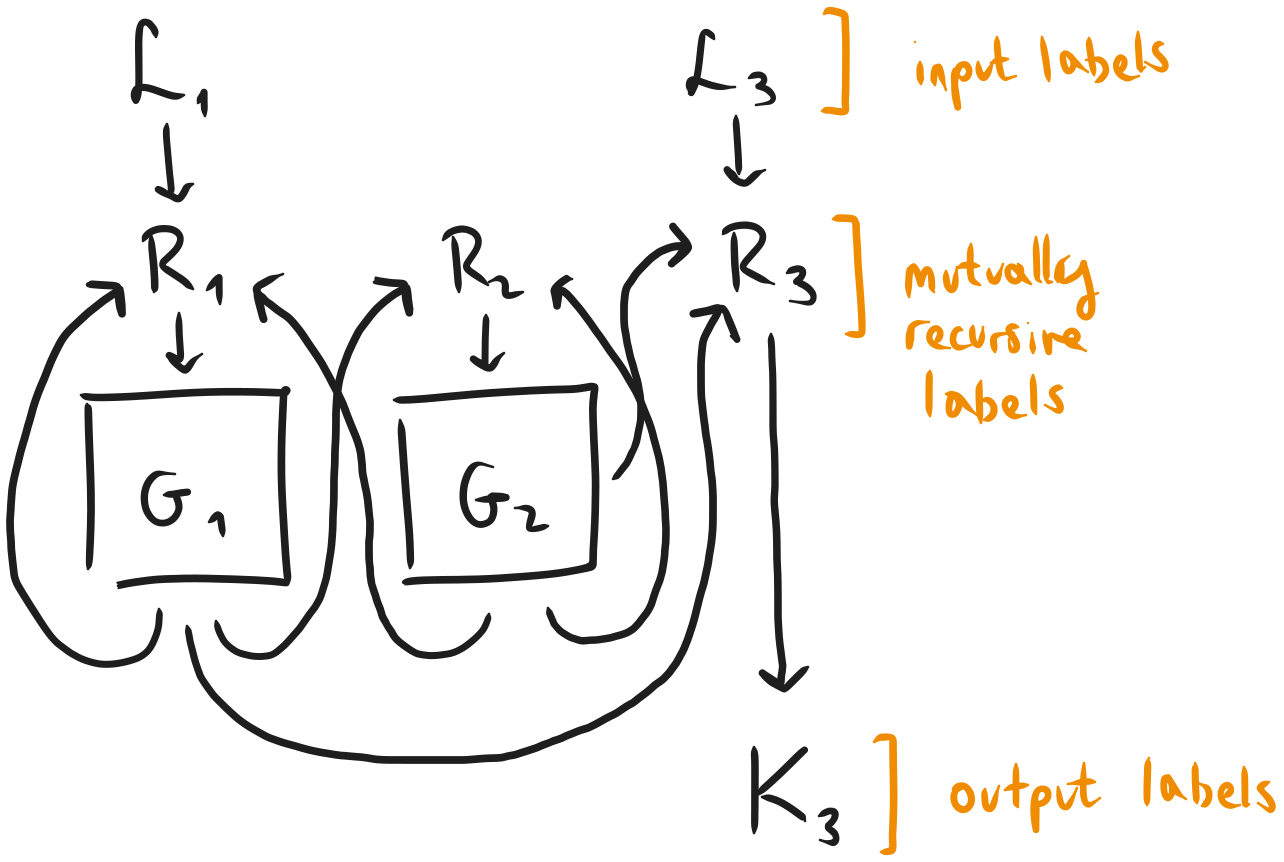
Finally, a control-flow graph $G$ can be viewed as a set of mutually-recursive basic blocks taking a label context of entry points $\mathcal{L}$ to a label context of exit points $\mathcal{K}$, as in the following picture:

Representing $G$ as a finitely-supported map from labels $\ell$ to basic blocks $\beta$, the judgement for this might look like the following:

with a typing rule of the form

This rule is a bit complex, so let’s break it down:

• We postulate the existence of a recursive label context $\mathcal{R}$ such that:
• $\mathcal{L}$ weakens $\mathcal{R}$, i.e. for every label $\ell \in \mathcal{L}$, $\mathcal{L}(\ell) \leq \mathcal{R}(\ell)$. In particular, $\mathcal{R}$ is allowed to map labels not in $\mathcal{L}$ to arbitrary contexts.
• For every $ℓ$ in $G$, if $\mathcal{R}(\ell)$ are live on entry to $G(\ell)$ then all branches out of $G(\ell)$ have the appropriate contexts in $\mathcal{R}$ live.
• For every $ℓ$ in $\mathcal{R}$ not in $G$, $\mathcal{R}(\ell)$ is just a weakening of the corresponding output label $\mathcal{K}(\ell)$. Note the rule would be equally powerful if we required an equality $\mathcal{R}(\ell) = \mathcal{K}(\ell)$

We can similarly state a weakening lemma

and frame rule (assuming all labels in $\mathcal{N}$ are fresh!)

SSA

So far, our type system and grammar applies to 3-address code in general, rather than SSA specifically, and in particular much of our semantics work and optimizations work in this setting as well. We can now define SSA form as a property of 3-address code: a piece of 3-address code is said to be in SSA form if every variable is assigned to exactly once.

Conversion to SSA form, for straight-line code, is just variable renaming:

x = x + 3;
y = x + 2;
x = 3 + y;
y = x + y;

becomes

x1 = x0 + 3;
y0 = x1 + 2;
x2 = 3 + y0;
y1 = x2 + y0;

The reason we are interested in SSA is that this property allows for substitution: we can safely substitute all occurences of x2 with 3 + y0, for example, whereas previously we would have to keep control-flow in mind. In general, the ability to analyze the previous values of variables, and do algebra with them, makes a huge class of analysis passes and optimizations much easier to implement.

In the presence of branching, however, converting to SSA gets a bit more complicated: given

^entry:
    x = 5;
    ite p ^left ^right
^left:
    x = 3 + x
    br ^end
^right:
    x = 4
    br ^end
^end:
    x = 3 + x

trying to simply number our variables leaves us with the following:

^entry:
    x0 = 5;
    ite p ^left ^right
^left:
    x1 = 3 + x0
    br ^end
^right:
    x2 = 4
    br ^end
^end:
    x3 = 3 + x?

In particular, it is dependent on control-flow whether x1 or x2 is used in the definition of x3. The solution to this issue is to introduce parameters for basic blocks, as follows ¹

^entry:
    x0 = 5;
    ite p ^left ^right
^left:
    x1 = 3 + x0
    br ^end(x1)
^right:
    x2 = 4
    br ^end(x2)
^end(x3):
    x4 = 3 + x3?

To take into account parameters, we can change our definition of label contexts to map labels $\ell$ to pairs $(\Gamma, (A_i)_i)$ of contexts $\Gamma$ and tuples of parameters $A_i$.

We might then modify our typing judgement for blocks as follows:

Here, we define $(\Gamma, (A_i)_i) \leq (\Delta, (B_i)_i) \iff \Gamma \leq \Delta \land \forall i, A_i = B_i$.

Similarly, control flow graphs must be modified to map labels $\ell$ to pairs $((x_i)_i, \beta)$ of tuples of variable names $(x_i)_i$ and basic blocks $\beta$ parametrized the $x_i$s.

Our typing rule for CFGs then becomes

Note that these typing rules are still for 3-address code (extended with basic block parameters), and well-typed programs do not necessarily have to be in SSA.

Adding an Expression Language

At this stage, we can define a predicate determining whether a control-flow graph is in SSA form quite easily: all we need to do is check that for every basic block $\Gamma, (x_i : A_i)_i \vdash \beta \rhd \mathcal{L}$, $\beta$ does not overwrite any variables which were live on input to $\beta$, i.e., in $\Gamma$ or $\{x_i\}$. Unfortunately, writing down equations about substitutions and rewrites, which was the point of moving to SSA in the first place, is still quite a pain in our setting. For example:

• Propagating a constant binding $\mathsf{let}\;x = c$ knowing that $x$ is not redefined is sound (the program being in SSA implying no variable is redefined), since constants cannot appear as arguments to functions in our simple grammar, we need to instead create many constant bindings $\mathsf{let}\;x_u = c;$ for each use $u$ of $x$ we want to replace, which at least temporarily just seems to make our program more complicated. We also, of course, need to deal with fresh variables.
• We have to suffer a bit to perform algebraic optimizations such as simplifying $x = y - 5; z = x + 5$ to $x = y - 5; z = x$, since we cannot directly rename variables.
• We don’t know which operations we can safely substitute: an add is fine, but a call to print isn’t… and oftentimes, neither is a div due to risk of undefined behaviour on division by zero.
• We might want to detect more complicated multi-layer patterns, using advanced techniques such as E-graph rewriting

In short, introducing instructions is a pain, and matching patterns of pure operations is a pain. This in particular makes writing a formal substitution theorem a pain. To address this, we can introduce a simple expression language, to replace operations, having the following typing judgement

This judgement says that, in the context $\Gamma$, the expression $a$ has type $A$ and effect $\epsilon$. In general, our effects form a lattice, but for now, it is enough to consider pure expressions with effect $\bot$ and impure expressions with effect $\top$; only substitutions of the latter are semantically sound! We will also extend contexts $\Gamma$ to map variables $x$ to pairs $(A, \epsilon)$ of a type and an effect: this allows us to reason about terms, bodies, blocks, and CFGs with free variables of impure type, allowing us to reason about the syntactic soundness of rewrites. ²

Note that, to effectively deal with multiple return values, we simply ban them, instead introducing product types $(A_1 \times ... \times A_n)$, which we will write $\Pi_i A_i$. We also annotate each expression with an effect $\epsilon$.

We postulate the expected typing rules:

These satisfy the expected weakening lemma

We must now modify our typing judgement for bodies to differentiate between binding a variable and unpacking:

and our judgement for blocks and control-flow graphs to deal with the fact that only single arguments are now permitted

Note that label contexts $\mathcal{L}$ are now mappings $\ell \mapsto (\Gamma, A)$, i.e., there is now only a single parameter type. Similarly, we modify the rules for CFGs as follows:

where control-flow graphs $G$ are now mappings $\ell \mapsto (x, \beta)$. Weakening and label-weakening can be shown to hold exactly as before.

Note that this system is obviously isomorphic to the original, with expressions just introducing anonymous temporary variable bindings and renamings.

Adding a Terminator Language

Similarly, it greatly simplifies label substitutions if we also have a language for terminators; this also allows us to avoid introducing spurious basic blocks consisting only of conditional branches, especially since we do not, in our simple language, have a switch-statement. In particular, we introduce the following judgement, analogous to that for blocks, with the following obvious rules:

Blocks can then be typed as follows:

Once again, this change doesn’t add any new expressive power to our system: we can convert a CFG in the new system to a CFG in the old system by just introducing basic blocks with temporary names to the CFG in the obvious way. One other useful property this system has is that it typechecks a strict superset of the syntax the previous system does.

Substitution

Now that we have an expression language, we can attempt to formalize substitution, which can then be used to formalize a wide variety of optimizations such as loop hoisting and constant propagation.

We begin by defining a substitution $\sigma : \Gamma \to \Delta$ to be a map from variables to terms such that $\forall (x, A, \epsilon) \in \Delta. \Gamma \vdash_\epsilon \sigma(x) : A$. In particular, we say $\sigma$ is pure if $\forall (x, A, \epsilon) \in \Delta. \Gamma \vdash_\bot \sigma(x) : A$.

Stating substitution for expressions is quite straightforward: if $\sigma : \Gamma \to \Delta$, then

with this substitution semantically sound if $\sigma$ is pure. Unfortunately, even graduating to bodies makes things a lot more complicated. One issue is that, since we are working in a named setting, it is nontrivial implement capture-avoiding substitution, since the usual approach of renaming bound variables to fresh names won’t work if implemented as the names of bound variables are visible on the right-hand side of the judgement for bodies. More concretely, given the body

let z = 3;
let x = y;

and the substitution $y \mapsto 3 + z$, we might try writing the substitution as

let z0 = 3;
let x = y + z;

except now $z$ does not have the appropriate value ($3$) at the end of the body! So we instead need to write something like

let z0 = 3;
let x = y + z;
let z = z0;

Instead, we’ll do what real SSA-based compilers often do and simply use naive, non-capture avoiding substitutions. This of course mans that a substitution is only valid if

Another complication is, considering the case where $\sigma : \Gamma' \to \Gamma$, it is unclear what $\Delta'$ should be in

This is because some variables in $x \in \Delta$ may come from $\Gamma$ (rather than being newly defined in the body), but not be contained in $\Gamma'$, being instead defined as $\sigma(x)$.

We hence introduce a new judgement

where $\Delta$ consists of exactly the variables defined by $b$, with rules

and note that

This new judgement then respects substitution, with substitution lemma

We can proceed similarly for basic blocks and CFGs, but we have to do a whole lot more fiddling with names, taking thousands of lines of Lean to formalize! It seems clear that, should we want to be able to effectively state this and more complicated theorems (such as label-substitution), we will need a more convenient representation of SSA.

Formalization

We have now obtained a system which is essentially the same as that formalized in freyd-ssa, except for a few small details, which we will go over now.

freyd-ssa defines types inductively as follows:

In particular, types are generated freely from a set of base types $X$. For simplicity, we only define pairs of types $A \times B$, and an explicit unary type $\mathbf{1}$; these can simulate $n$-ary pairs $\Pi_i A_i$ by defining, e.g., $\Pi_{i = 1}^nA_i = A_1 \times \Pi_{i = 2}A_i$. We also include a builtin boolean type $\mathbf{2}$.

Hence, in particular, our term language only defines binary pairs and a constant $()$ of type $\mathbf{1}$:

Similarly, our grammar for bodies only allows binary destructuring:

One other change is that our rules for CFGs are a little bit more convoluted: we define $\mathcal{L} \vdash' G \rhd \mathcal{K}$ using the following much less intuitive rules:

where $G, \ell(x) \Rightarrow \beta$, as expected, denotes changing $G(\ell)$ from undefined to $(x, \beta)$, with CFG well-typedness then given by

The reason for this had to do with wanting a more inductive semantics; in retrospect, I can’t think of why exactly we went for this this at the moment, but that’s what was formalized and we have to be honest! This is roughly equivalent to the formulation given above, though it provides a bit more power, since “dead” code, i.e. $\ell$ not reachable from the entry context, does not need to typecheck.

Adding Coproducts

One of the design goals for freyd-ssa was to keep things as conventional as possible. Hence, we did not support coproducts, and instead only provided a Boolean type $\mathbf{2}$. However, effectively reasoning about coproducts can not only allow us to perform various interesting optimizations, especially when the source language supports them, but also makes it a lot easier to prove category-theoretic properties of our semantics. So, in debruijn-ssa, we choose to support them.

In particular, our types are now given by the grammar

and terms are extended in the obvious manner:

For control-flow, we replace $\mathsf{ite}$ with a $\mathsf{case}$ terminator, which binds variables, similarly to pattern-matching:

Note that we can easily simulate booleans in this setting by defining

Explicit Scoping and De-Bruijn Indices

Now that we’ve seen how difficult it is to state substitution when using names as above, we want to develop an inductive representation of SSA which is easier to reason about, while at the same time isomorphic to our original language. To do this, we have to think carefully about how variables and labels are scoped in SSA.

Dominator Trees

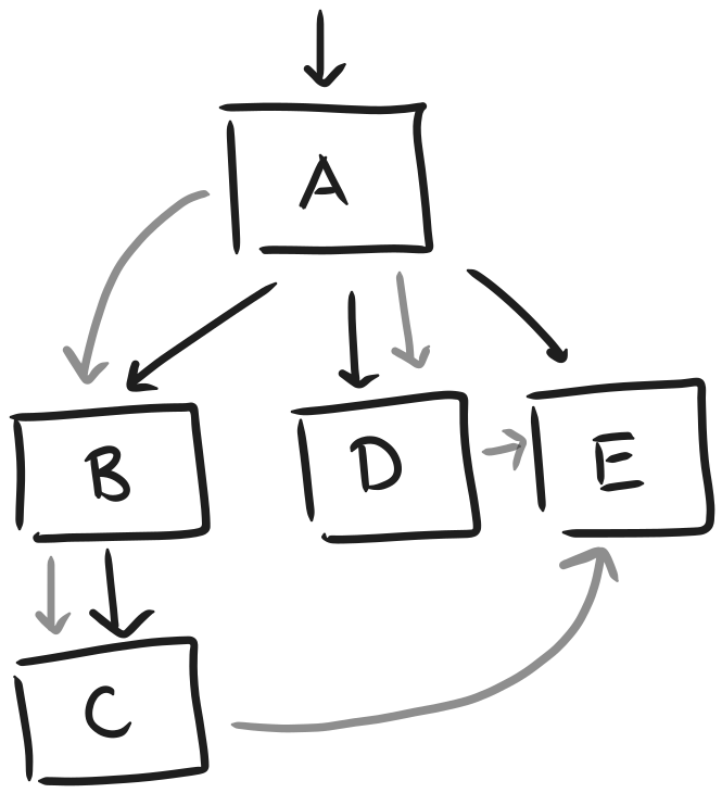
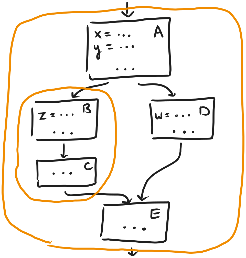
Consider the control-flow graph below:

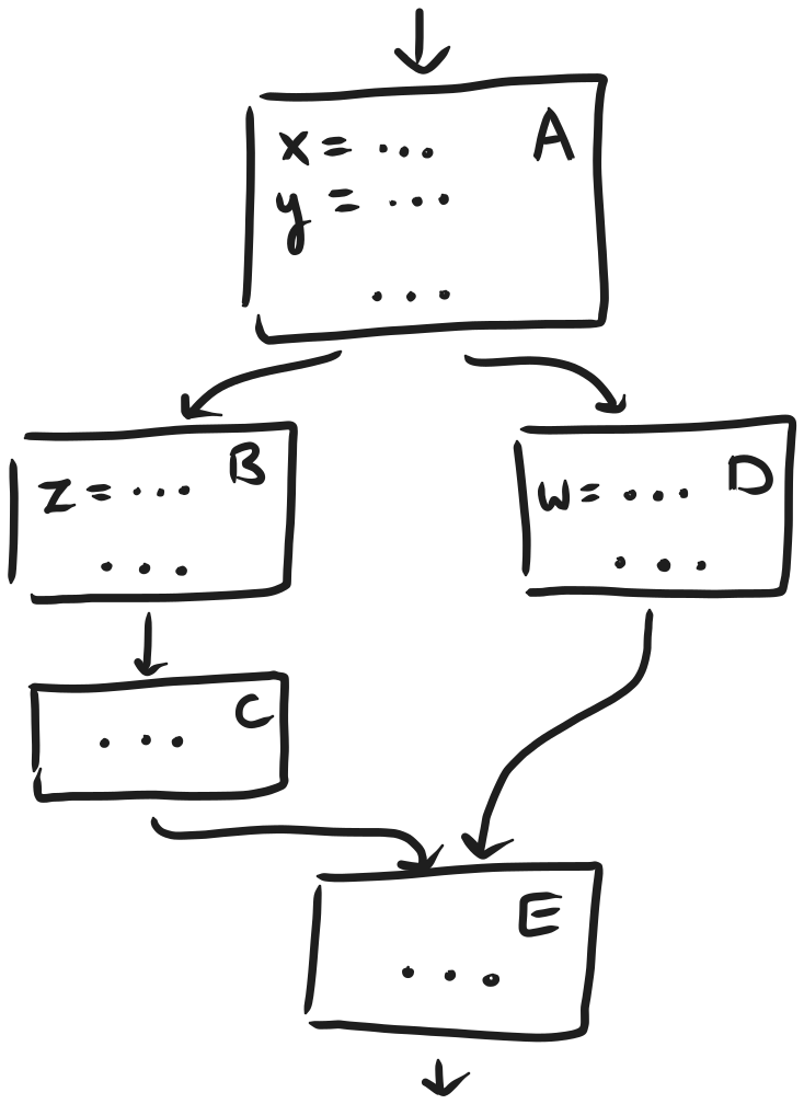
Here, the entry block, $A$, defines variables $x, y$, and then jumps to either $B$ or $D$. $B$ defines $z$ and then jumps to $C$ unconditionally, which then jumps to $E$, whereas $D$ defines $w$ and then jumps straight to $E$.

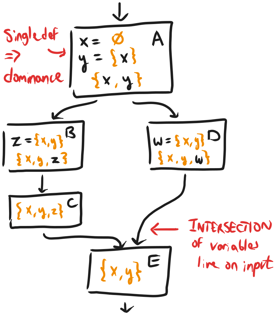
We might want to ask ourself which variables can be used, i.e. are live, at each point in the program. We can perform a liveness analysis as follows:

• At the very beginning of the program, the definition of $x$ in $A$, no variables are yet live
• Immediately afterwards, at the definition of $y$, only $x$ is live
• On entry to $B$, at the definition of $z$, $x, y$ are live, while on entry to $C$, $x, y, z$ are live
• Similarly, on entry to $D$, at the definition of $w$, $x, y$ are live
• On the other hand, only $x, y$ are live on entry to $E$. This is because
  • $z$ cannot be live, since if we came from $D$, it would be undefined
  • $w$ cannot be live, since if we came from $C$, it would be undefined

In other words, the live variables on entry to any basic block are the intersection of the live variables on exit from any basic block which jumps to that basic block. This gives us a recipe for building a dataflow analysis to compute live-variable sets, one of the fundamental building blocks of classical techniques for building compilers for 3-address code.

If our program is additionally in SSA, however, things are a bit simpler, and more interesting. Note that a variable $x$ is live at the entry to a given basic block $B$ if and only if all paths to that block through the control-flow graph reaching $B$ go through at least one place where the $x$ is defined. If our program is in SSA, each variable $x$ is defined at exactly one point $A$, so a $x$ is live if and only if all paths reaching $B$ through the control-flow graph go through $A$, i.e., in graph-theory speak, if $A$ dominates $B$. Note that dominance is a transitive and reflexive relation.

Of course, since in general $x$ is not visible in its own definition (or for variables defined before $x$ in the same basic block $A$!), we want to consider whether $A$ strictly dominates $B$, i.e., whether $A$ dominates $B$ and $A ≠ B$; if this is the case, we can be certain all variables defined in $A$ are live on reaching $B$.

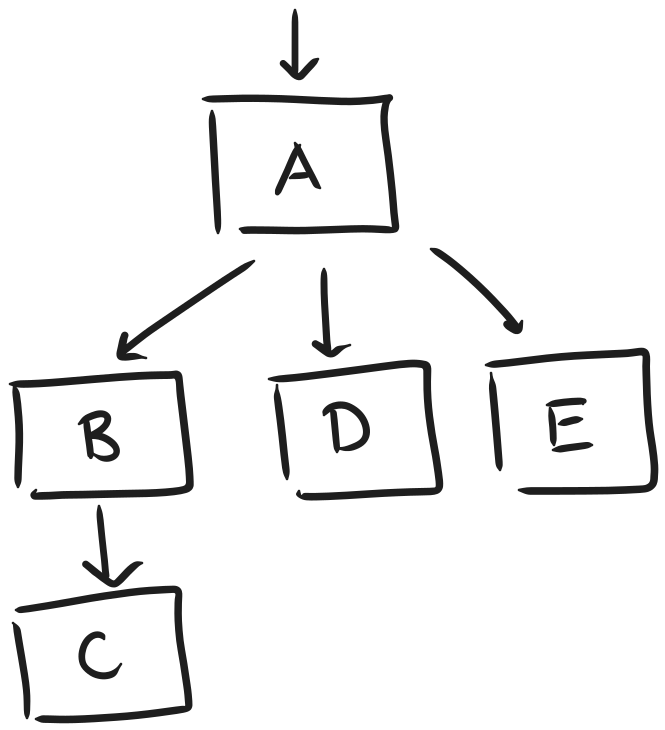
In general, the dominance tree of a control-flow graph encodes this relation; it has:

• Nodes for each basic block in the control-flow graph
• An edge from node $A$ to $B$ if $A$ strictly dominates $B$ and there is no intermediate node $A'$ such that $A$ dominates $A'$ and $A'$ dominates $B$.

For example, the dominance tree of the example control-flow graph from before can be written:

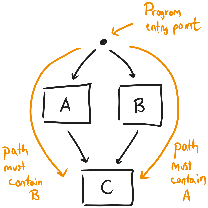
As long as all nodes in the control-flow graph are reachable (in the graph-theoretic sense, even if control flow will never actually reach them!) from the program entry point, this is indeed always a tree; this property always holds after unreachable code elimination. To see why, consider the case where $A$ and $B$ both strictly dominate $C$. It suffices to show that $A$ dominates $B$ or $B$ dominates $A$. Assume that $A$ does not dominate $B$ and $B$ does not dominate $A$. Then there exists a path $p_A$ from the entry point to $A$ which does not reach $B$, and a path $p_B$ from the entry point to $B$ which does not reach $A$. It follows that all paths from $B$ to $C$ must reach $A$, as if there was a path $q$ which did not do so, then $p_B; q$ (where $;$ denotes path composition) would go from the entry point to $C$ without reaching $A$, yielding a contradiction. By symmetry, all paths $q$ from $A$ to $C$ must reach $B$.

We wish to show that there is no path $q$ from $A$ to $C$ or from $B$ to $C$. To do show, we prove that any such path must be infinitely long, i.e., for all $n$, it must be longer than $n$. We proceed by induction:

• Inductive hypothesis $P(n) := ∀k \leq n.$ “the path cannot be of length $\leq n$”
• $P(0)$: The path cannot be of length 0, since $A, B ≠ C$
• $P(n) \implies P(n + 1)$: if the path is of length $n + 1$, then it must go through either $A$ or $B$ after $0 < k < n + 1$ steps. But the sub-path from this point to $C$ is of length $(n + 1) - k \leq n$, yielding a contradiction.

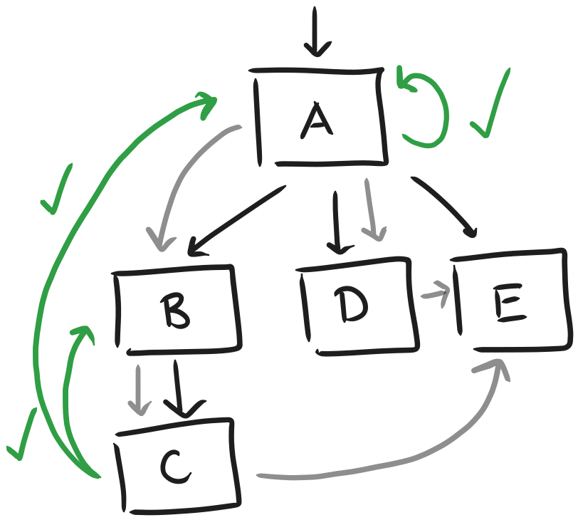
Going back to the dominance tree we drew, we can add our control-flow edges back in in grey:

Let’s consider what kind of control edges we could add without changing the dominance structure. As we would hope, it is always OK to add control edges to direct descendants in the dominance tree:

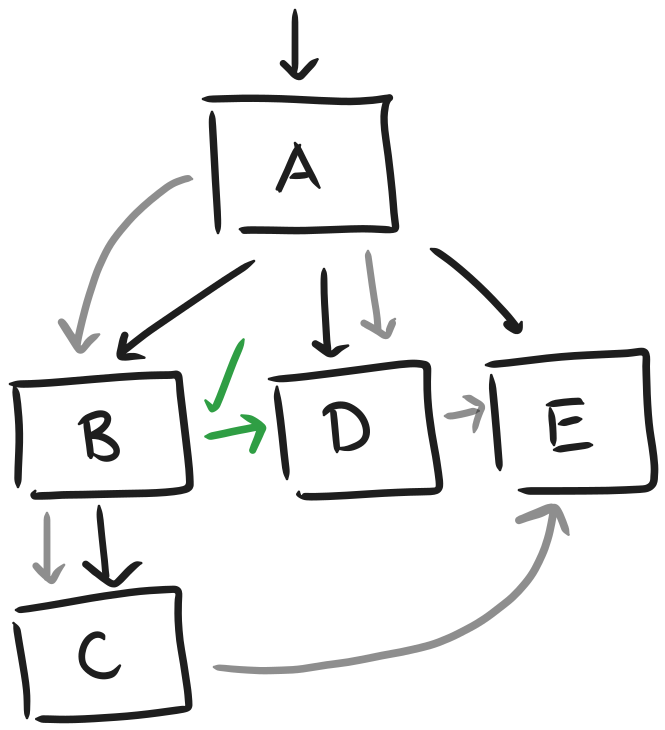
Similarly, control edges between siblings seem to be fine:

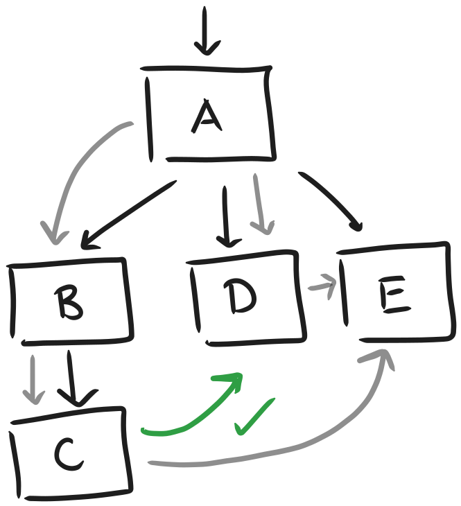
It also seems to be fine to add control edges to the siblings of our ancestors, our “uncles”:

As well as to parents, grandparents, and ourselves

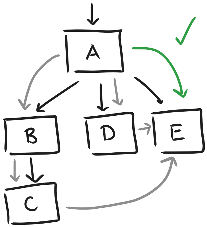
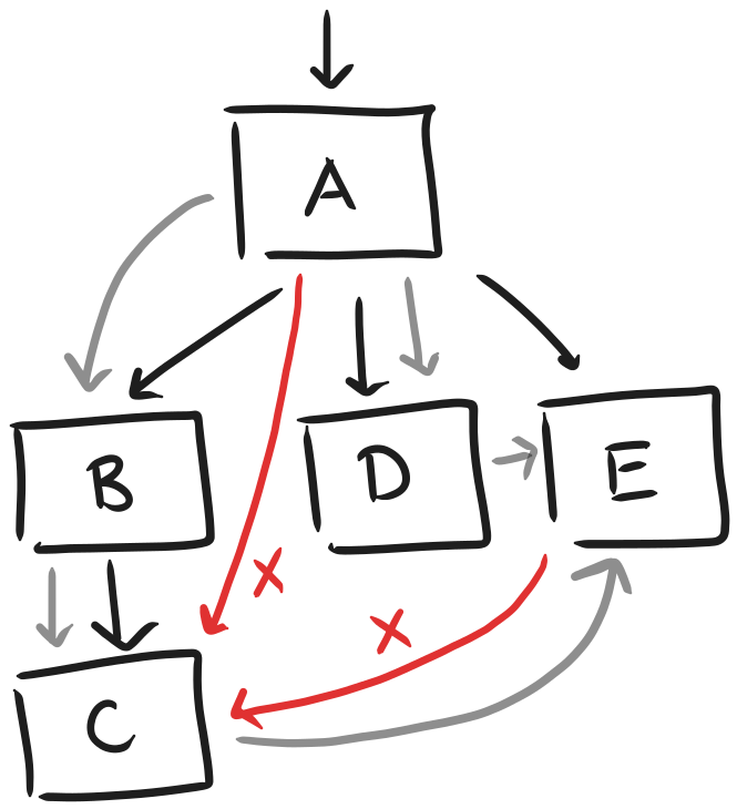
But edges to our grandchildren would violate the dominance structure, since, for example, adding an edge from $A$ to $C$ would create a path from the entry to $C$ which does not reach $B$.

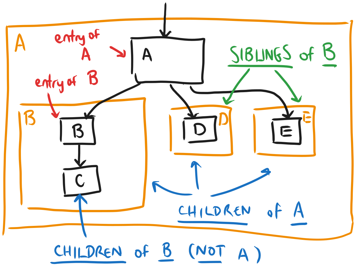
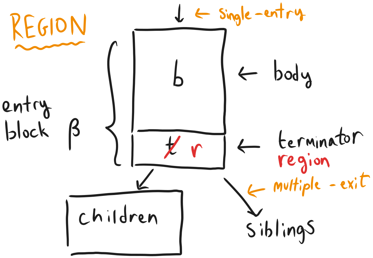
This points to an organization of our program into regions, such that

• Each node in the dominance tree is the entry block of its region
• The children of that node are the region’s children
• All a node’s descendants, including the node itself, are considered inside that node’s region

Now, the correctness rule becomes very simple: “every control-flow edge going from the outside of a region to the inside of a region must target the entry-block of that region.”

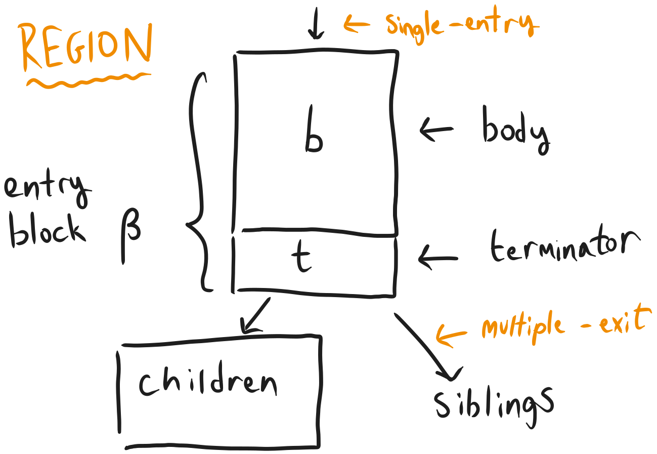
We might hence represent a region as a basic block, followed by a list of child regions which only this entry block can call (the entry blocks of)

In particular, since liveness is now taken care of by the structure of the CFG itself, we no longer need to keep track of live variable sets in label contexts, and hence can define them to simply be maps $\mathcal{L}$ from labels to parameter types $A$.

We may hence introduce the syntactic class of regions $l, r$ with typing rule

Let’s break this rule down: given that

• The body $b$, given variables $\Gamma$ live on entry, has variables $\Delta$ live on exit
• The terminator $t$, given variables $\Delta$ live on entry, jumps to either children $\mathcal{R}$ or an external label from $\mathcal{L}$
• For each child $\ell\;x_\ell \Rightarrow G_\ell$, if $G_\ell$ is a region which, having live variables $\Delta, x_\ell : \mathcal{R}(\ell)$ on entry, jumps to either siblings $\mathcal{R}$ or an external label from $\mathcal{L}$
• Then $\mathsf{reg}\;(b;t)\;(\ell\;x_\ell \Rightarrow G_\ell)_\ell$ is a region which, having live variables $\Gamma$ on entry, jumps to a label in $\mathcal{L}$, with
  • Entry block $(b;t)$
  • Children $(\ell\;x_\ell \Rightarrow G_\ell)_\ell$

The rules for terminators are left essentially unchanged:

The astute reader may notice that in both this typing rule and the above diagram, the entry block cannot necessarily call itself. However, any region other than the root of the CFG will have its own address available to jump to as a sibling; consequently, the natural way to represent a programs CFG is by nesting in a dummy outermost region with an unconditional jump to the program’s entry point as entry block.

Recovering a standard control-flow graph from such a region is simple: all one needs to do is to “flatten” the syntax tree as follows (assuming all labels are fresh for simplicity):

Graphically, this simply corresponds to “erasing the region boundaries”, here in orange:

De-Bruijn Indices

One of the major advantages of this representation is, having gotten ride of the cumbersome original “context of contexts” definition for label contexts $\mathcal{L}$, we now have a clear system of variable scoping, following the structure of the dominance tree. This allows us to use de-Bruijn indices for variables, rather than names. Since labels also obey this scoping system, we may use de-Bruijn indices for them too. For simplicity, however, we will use names to describe the typing rules in this article.

At this point we’ve described the BBRegion data structure in debruijn-ssa, except that our expression language is extended into a term language, which we will elaborate on later.

Removing Bodies

Substitution is much easier to state in this new framework.: in particular, since we now have a strict variable scoping discipline, we may use capture-avoiding substitution, such that, in particular, for any substitution $\sigma : \Gamma \to \Delta$, we have

That said, actually proving it is still slightly irritating, since of course our rules for bodies remain unchanged. Thankfully, things now become much easier if, analogously to our previous transformation for basic blocks, we fuse bodies and regions, as follows:

This gives us essentially the TRegion data structure in debruijn-ssa; substitution and weakening hold just as before.

How to Recover SSA

We can state the isomorphism between TRegion and BBRegion as follows:

where

and

where

Structured Branching Control-Flow

We already have a pretty decent inductive representation for SSA at this point. One additional thing we want to be able to reason about effectively, however, is control-flow graph manipulations, such as composing control-flow graphs by connecting their inputs and outputs.

One way to state such rewrites effectively is through label substitution, in which branches $\mathsf{br}\;\ell\;a$ are replaced with arbitrary code parametrized by $a$. Unfortunately, this is a bit unwieldy when terminators can only contain control-flow. Thankfully, it’s straightforward to generalize this problem away: all we need to do is merge terminators and regions, as follows:

Doing this gives us the Region data structure in debruijn-ssa, but see Term.

Intuitively, all we’ve done is generalize the old region data structure as follows:

Note that this grammar typechecks a strict superset of all valid TRegions, which can always be reached by semantics-preserving rewrites such as

For brevity, we will omit the full normalization algorithm.

Label substitution

We can now define a label substitution $\sigma$ to be given by a map from labels $\ell$ to regions $r$ parametrized by a free variable $x_\ell$. We say such a substitution $\sigma : \Gamma;\mathcal{L} \to \mathcal{K}$ is well-typed in $\Gamma$ if

In this case, we have that

where $[\sigma]r$ is capture-avoiding (for both labels and variables; this is much easier to state with de-Bruijn indices!) substitution of labels defined as follows:

Introducing a Term Language

We now come to the final change required for some of the optimizations we would like to do: generalizing our expression language to a term language. It turns out that sometimes we want to splice and merge a control-flow graph based on algebraic rewriting; the simplest way to do this is to allow (branching) control-flow to be represented as part of our algebraic expression language, as follows:

Again, this grammar can represent strictly more programs than those based on the old expression language. Given a region parametrized by terms, we can rewrite it to a region valid in the old grammar using obvious semantics-preserving rewrites such as